import pandas as pd
import numpy as np
import matplotlib.pyplot as plt
import matplotlib.animation
import IPython
import sklearn.tree

#---#
import warnings
warnings.filterwarnings('ignore')의사결정나무 | 작동원리
tree
의사결정나무가 작동하는 원리에 대해서 알아보자!
해당 포스트는 전북대학교 통계학과 최규빈 교수님의 강의내용을 토대로 재구성되었음을 알립니다.
1. 라이브러리 imports
2. 원리
A. max_depth
얼만큼 깊게 나눌 것이냐???를 결정한다. 이 말을 이해해보자.
- Data
np.random.seed(43052)
temp = pd.read_csv('https://raw.githubusercontent.com/guebin/DV2022/master/posts/temp.csv').iloc[:,3].to_numpy()[:100]
temp.sort()
eps = np.random.randn(100)*3 # 오차
icecream_sales = 20 + temp * 2.5 + eps
df_train = pd.DataFrame({'temp':temp,'sales':icecream_sales})
df_train| temp | sales | |
|---|---|---|
| 0 | -4.1 | 10.900261 |
| 1 | -3.7 | 14.002524 |
| 2 | -3.0 | 15.928335 |
| 3 | -1.3 | 17.673681 |
| 4 | -0.5 | 19.463362 |
| ... | ... | ... |
| 95 | 12.4 | 54.926065 |
| 96 | 13.4 | 54.716129 |
| 97 | 14.7 | 56.194791 |
| 98 | 15.0 | 60.666163 |
| 99 | 15.2 | 61.561043 |
100 rows × 2 columns
## 일단 늘 했던 것처럼...
## step1
X = df_train[['temp']]
y = df_train['sales']
## step2
predictr = sklearn.tree.DecisionTreeRegressor(max_depth=1) ## NEW!
## step3
predictr.fit(X,y)
## step4 -- pass
# predictr.predict(X) DecisionTreeRegressor(max_depth=1)In a Jupyter environment, please rerun this cell to show the HTML representation or trust the notebook.
On GitHub, the HTML representation is unable to render, please try loading this page with nbviewer.org.
DecisionTreeRegressor(max_depth=1)
- 결과를 시각화
plt.plot(X, y, 'o', alpha = 0.5, label = 'True')
plt.plot(X, predictr.predict(X), '--', label = 'Predicted')
plt.legend()
plt.show()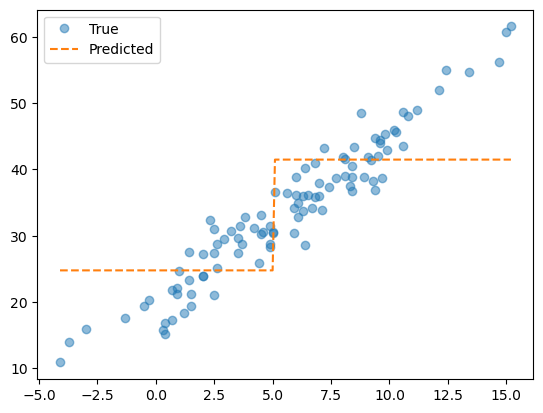
5.0정도를 기준으로 계단이 뚝 끊긴 모습이다.
기존에는 막 이래저래 왔다갔다 하면서 오버피팅이 되는 모습이었는데, max_depth = 1옵션을 추가하니 뚝 끊겨서 값이 산정된다. 어떤 원리인지 알겠는가…?
- tree 시각화
sklearn.tree.plot_tree(predictr)[Text(0.5, 0.75, 'x[0] <= 5.05\nsquared_error = 111.946\nsamples = 100\nvalue = 33.973'),
Text(0.25, 0.25, 'squared_error = 34.94\nsamples = 45\nvalue = 24.788'),
Text(0.75, 0.25, 'squared_error = 49.428\nsamples = 55\nvalue = 41.489')]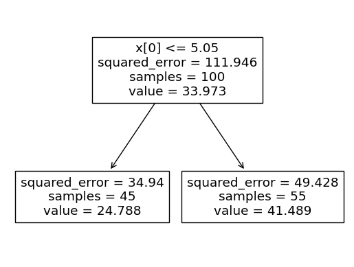
의사결정나무는 이런 방식으로 적합을 한다!!
적당한 \(x\)값을 기준으로 데이터를 나눈 뒤, 각 구간에 해당하는 녀석들의 \(y\)값 평균으로 예측해버린다!
## 그럼 max_depth가 2라면???
## step1
X = df_train[['temp']]
y = df_train['sales']
## step2
predictr = sklearn.tree.DecisionTreeRegressor(max_depth=2)
## step3
predictr.fit(X,y)
## step4 -- pass
# predictr.predict(X)

plt.plot(X, y, 'o', label = 'true', alpha = 0.5)
plt.plot(X, predictr.predict(X), '--', label = 'predicted')
plt.legend()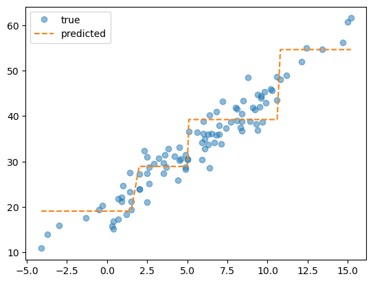
방금 전의
tree_plot을 기억하는가? 거기서 한 번 더 내려온 것(한 단계 더 깊게 적합)이max_depth = 2이다!
### B. 애니메이션
아직도 잘 감이 오지 않는다면,
animation을 이용해max_depth에 따른 예측값의 변화를 시각화해보자.
fig = plt.figure()<Figure size 640x480 with 0 Axes>def func(frame):
ax = fig.gca()
ax.clear()
predictr = sklearn.tree.DecisionTreeRegressor(max_depth = frame+1)
predictr.fit(X, y)
ax.plot(X, y, 'o', alpha = 0.5, label = 'True')
ax.plot(X, predictr.predict(X), '--', label = 'Predicted')
ax.set_title('max_depth = {}'.format(str(frame+1)))ani = matplotlib.animation.FuncAnimation(
fig,
func,
frames = 10
)
display(IPython.display.HTML(ani.to_jshtml()))
max_depth의 값이 커질수록 계단의 구간이 많아지더니 점을 따라가기 시작했다…
코드를 쉽게 쓰기 위해서 func에다 fitting하는 것까지 넣어줬지만, 원래는 외부에서 fitting된 녀석을 넣어주는 게 리소스 절감에 용이하긴 하다…
C. 분할을 결정하는 기준?
그럼 그 계단의 경계는 어떻게 결정되는 걸까?
predictr.score(X, y)0.8561424389856722y_hat = predictr.predict(X)
sklearn.metrics.r2_score(y, y_hat) ## 딱히 라이브러리를 들여오지 않아도 나오네...0.8561424389856722회귀모형이 전체 변동 중 얼마만큼을 설명했는지를 나타내는 \(R^2\)를 좋은 분할을 판단하는 기준으로 사용한다.
즉, 가능한 계단의 경계값들 중 \(R^2\)이 가장 높은 값이 분할로 결정된다!!
- 이 과정을 구현해보자.
def fit_predict(X, y, c) :
    """
    X와 y, 분할할 구간을 넣어주면 max_depth = 1일 때의 구간에 따른 예측값을 반환하는 함수.
    """
    X = np.array(X).reshape(-1)  ## 1차원으로 깨줌
    y = np.array(y)
    yhat = y*0  ## 초기값 배정
    yhat[X<=c] = y[X<=c].mean()  ## bool list로 슬라이싱
    yhat[X>c] = y[X>c].mean()

    return yhat
yhat_bad = fit_predict(X, y, 1)
yhat_good = fit_predict(X, y, 5)
fig, ax = plt.subplots(1,2, figsize = (7,3))
ax[0].plot(X, y, 'o', alpha = 0.5)
ax[0].plot(X, yhat_bad, '--')
ax[0].set_title('R-squared = {}'.format(round(sklearn.metrics.r2_score(y, yhat_bad), 4)))
ax[1].plot(X, y, 'o', alpha = 0.5)
ax[1].plot(X, yhat_good, '--')
ax[1].set_title('R-quared = {}'.format(round(sklearn.metrics.r2_score(y, yhat_good), 4)))Text(0.5, 1.0, 'R-quared = 0.6167')
c의 값이 5일 때, \(R^2\)의 값이 더 클 뿐만 아니라, 예측한 값이 더 직관적으로 좋아보인다.
- 그래서 트리가 max_depth = 1일 경우 분할을 결정하는 방법! ~= 노가다…~
- 적당한 \(c\)를 고른다.
- 분할 \((-\infty, c), [c, \infty)\)를 생성하고
yhat을 계산한다. r2_score(y, yhat)을 계산하고 기록한다.- 상기 과정을 무한반복한 뒤,
r2_score(y, yhat)의 값을 가장 작게 만드는 \(c\)를 구간으로 택한다.
fit_predict??Signature: fit_predict(X, y, c) Source: def fit_predict(X, y, c) : """ X와 y, 분할할 구간을 넣어주면 max_depth = 1일 때의 구간에 따른 예측값을 반환하는 함수. """ X = np.array(X).reshape(-1) ## 1차원으로 깨줌 y = np.array(y) yhat = y*0 ## 초기값 배정 yhat[X<=c] = y[X<=c].mean() ## bool list로 슬라이싱 yhat[X>c] = y[X>c].mean() return yhat File: c:\users\hollyriver\appdata\local\temp\ipykernel_8144\486783211.py Type: function
cuts = np.arange(-5, 15)
fig = plt.figure()
def func(frame) :
    ax = fig.gca()
    ax.clear()
    yhat = fit_predict(X, y, cuts[frame])

    ax.plot(X, y, 'o', alpha = 0.5, label = 'True')
    ax.plot(X, yhat, '--', label = 'Predicted')
    ax.set_title(f'c = {cuts[frame]},  R-squared = {round(sklearn.metrics.r2_score(y, yhat), 4)}')
    ax.legend()
<Figure size 640x480 with 0 Axes>ani = matplotlib.animation.FuncAnimation(
fig,
func,
frames = len(cuts)
)display(IPython.display.HTML(ani.to_jshtml()))요런 느낌으로다가…
- 그럼 tree가 찾은 값 5.05를 우리가 직접 찾아보자.
cuts = np.arange(-5, 15, 0.001).round(5)
scores = np.array([sklearn.metrics.r2_score(y, fit_predict(X, y, c)) for c in cuts])
pd.DataFrame({'cut':cuts, 'score':scores}).plot.line(x = 'cut', y = 'score', backend = 'plotly')
cuts[scores.argmax()] ## R에서의 which()와 비슷한 느낌의 코드5.0
max_depth = 2인 경우는max_depth = 1의 결과로 발생한 2개의 조각을 각각 전체 자료로 생각하고,max_depth = 1일 때의 분할방법을 반복적용한다.
X.columns == ['temp', 'type']와 같은 경우라면, 설명변수를 하나씩 고정하여 각각 최적의 분할을 생성하고,r2_score관점에서 가장 우수한 설명변수를 선택한다.(즉, 가장 중요한 설명변수가 최우선적으로 고려된다.)
3. 토론
- 의사결정나무 vs 선형모형 !!!
- 의사결정나무의 장점
- 시각화가 유리하다, 설명력이 좋다.
- 특성(feature)의 중요도를 파악하기 용이하다(그야 가장 우수한 설명변수가
depth에 따라 최우선적으로 고려되니까.) - \(\textbf{y} \sim \textbf{X}\) 사이에 존재하는 비선형성을 간단히 모델링할 수 있다.
- 모형에 대한 가정들이 필요없다.(Nonparametric Model)
- 의사결정나무의 단점 : 오버피팅이 일어나기 너무 쉽다
- 자잘한 개념들(option)
최소 샘플 분할(min_samples_split)
- 노드를 분할하기 위한 최소 샘플 수.
- 과소적합(수를 줄임) 및 과적합(수를 늘림) 조절 가능
가지치기(Pruning)
- 트리의 불필요한 부분을 제거(아래로 뻗어나가는 가지 제거)하여 과적합 방지 및 모델 성능 향상에 도움.
정보 이득(Information Gain)
- 분할 전후의 엔트로피 차이를 측정(좀 많이 굉장히 어려운 개념임)
- 높은 정보 이득은 더 좋은 분할을 의미
지니 불순도(Gini Impurity)
- 노드의 순도 측정 지표, 낮은 지니 불순도는 높은 클래스 순도를 의미
결국 “트리를 어디까지 성장시킬래?”에 대한 이론적인 명확한 기술은 없다… Nonparametric Model이니까 정답이 없음…
의사결정나무를 응용한 다양한 방법(너무 많아요, 진짜)들이 개발되었고, 모든 방법들의 원리를 세세하게 파헤치는 건 비효율적이다…
그러한 다양한 방법들을 적당히 분류해보면 대체로 배깅, 랜덤포레스트, 부스팅 계열~(게다가 이중 여러가지를 포함하기도 함)~로 나뉜다. 앞으론 이 세 분류에 대한 공통적 아이디어를 파악해보도록 하자.